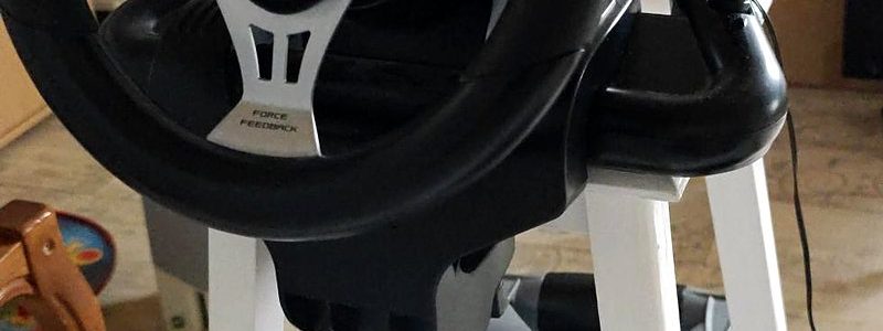
A 2007 Saitek wheel, one kernel oops, the I-Force protocol, and three proofs that some force feedback effects were never in the hardware.
Retour de Force: a 2007 Saitek R660GT vs. Linux Force Feedback
geekismes inside
A 2007 Saitek wheel, one kernel oops, the I-Force protocol, and three proofs that some force feedback effects were never in the hardware.
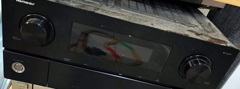
Every forum says the Ethernet port on a 2009 Pioneer receiver is dead. It was only waiting for DHCP, and behind it sat telnet and a full web remote.
A story box pulled from the trash, one regulator swap, and a home pipeline that tells bedtime stories about our own village, in my own cloned voice.
A 6 W netbook, two hidden power-limit registers and one lock bit: how a Celeron N3450 got 10 W and 61 percent more frames.
An orphaned Netgear NAS, a dying disk and a Debian rescue that ended with a 60-byte CRC loop, disks that finally sleep, and Samba reads nearly twice as fast.
If you have a cat, you know that sometimes his instincts push it to eat green eatable-looking plants, whatever they are, and whatever the consequences may be.
Spoiler: most of the time, it will require manual cleanup by the humans that happen to inhabit the same place.
It happens such a cat is living at my place.
And the Cat is often tempted by a plant which is not good for him.
So a solution had to be thought, as having a cat rejecting his stomach contents while you are in a middle of a meeting as you are working remotly from home is often a distractor not only for you but for your colleagues.
As a bonus, the device we would end up building could be used to prevent the cat from accessing other forbidden parts of the house, for example tables, kitchen hot plate..
Let’s break the habits of this blog, and show end results first!
Idea is to use tensorflow/OpenCV on a cheap raspberry 3B+ to detect the cat.
You can also follow this excellent tutorial on how to install tensorflow on the raspberry: https://github.com/EdjeElectronics/TensorFlow-Object-Detection-on-the-Raspberry-Pi
Some adaptations were required to get it to work, do not hesitate to contact me or post a comment here if you need help.
Simplest SSDLite MobileNet (which has learnt at 320×240) model was used so that it could run on the RP3B+, of course with « real » PC or a RP4 you could consider using one of the higher-res models available (check https://github.com/tensorflow/models/blob/master/research/object_detection/g3doc/tf2_detection_zoo.md).
After some tests, it appeared this model gave many false positives for categories others than cat, in particular « person » detection.
However, no false positives seen for the cat category, and some false negatives.
So that’s good enough to start plugging that detector to real-life world.
After having thought of putting some electronics/motor in a cheap, plastic water spray I already owned, similar to that:

I realised implementation would take time, multiple 3d-printing iterations (I have not seen any prior art in thingiverse) and my 3dprinter requiring maintainance + having little time to dedicate to that presently, I decided to go for another solution.
I also considered other similar experiments seen on the web such as that one: https://www.iot-experiments.com/cat-water-spray/ but I preferred to use an easy-to-refill solution.
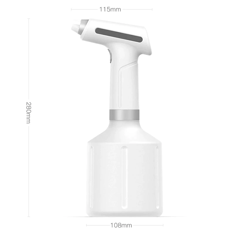
After searching a bit, I found this cheap electric water spray on Aliexpress (https://a.aliexpress.com/_An5jYW) :

Which – I imagined- would be easy to hack so that it could be controlled by the raspberry GPIOs rather than the original push button.
Be careful with screws hidden below the plastic adhesive on the sides of the spray.
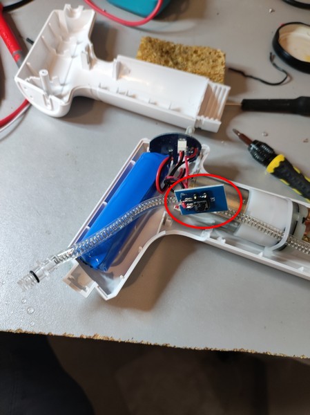
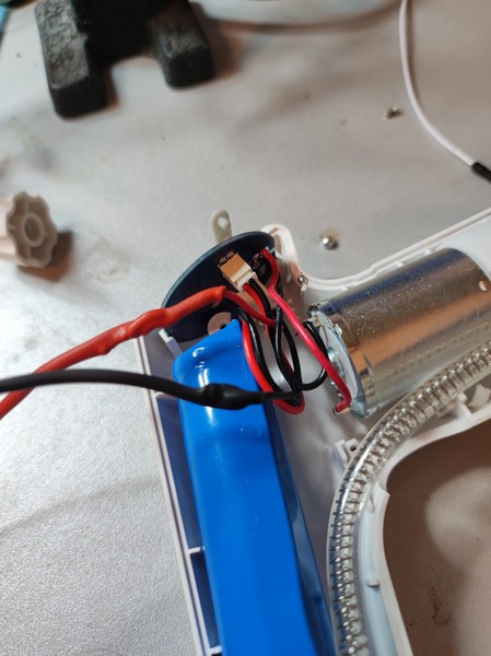
Then just use common sense to remove parts carefully, you should end up with that:
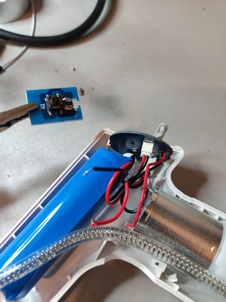
As you can see, one can easily see the button switch located in a dedicated PCB, link to the main logic PCB with black and red wires. Both wires are shortcut when button is pressed.
So we need to simulate that shortcut.
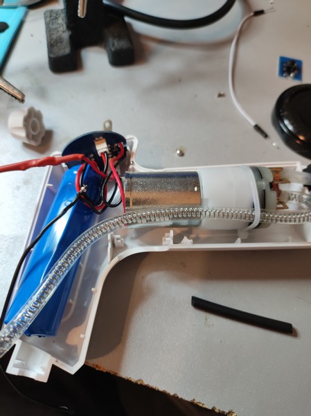
First, let’s get rid of the button part, to this end you can just unsolder the two wires. This option is preferable to cutting, as wires will be longer, which will be easier to handle what comes next.


So several options were considered:

+ : easy to put in place, very good isolation
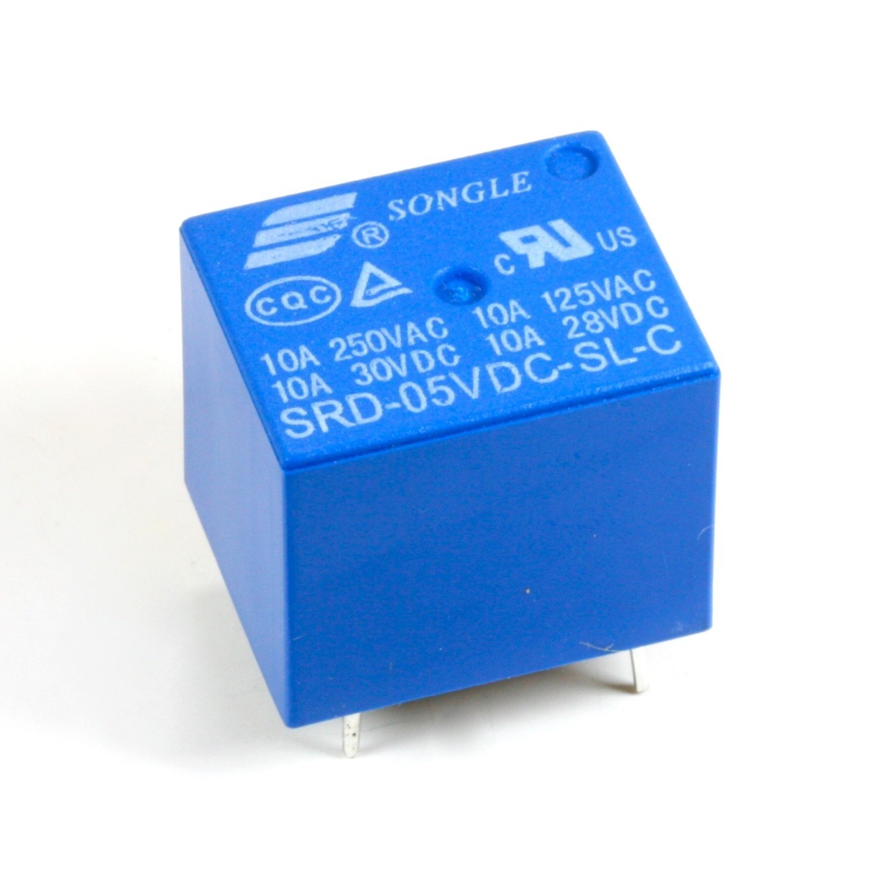
– : noisy when it operates, overkill for our application (very low current/voltage), not the least expensive, takes place (it’s big)

+ : very strong decoupling/isolation, quiet
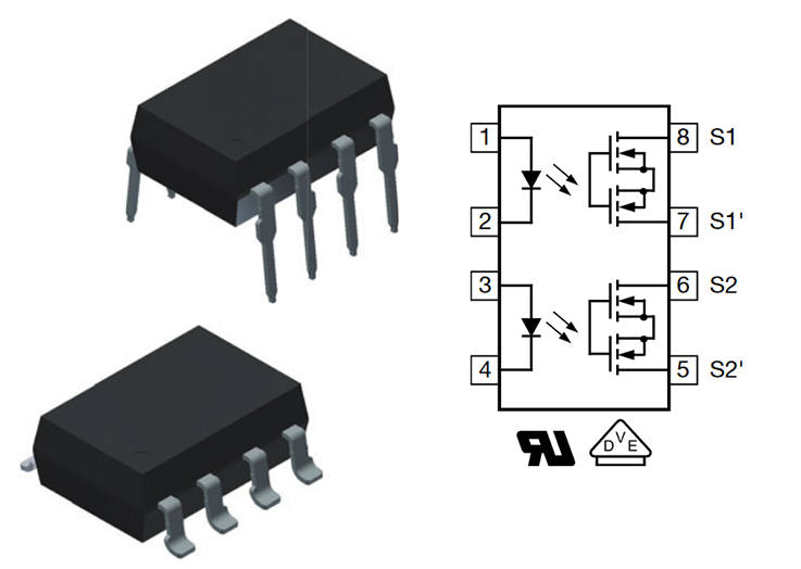
– : not the least expensive,

– : not the best isolation, but works fine in our case as we play with small voltage (the voltage difference between the 2 pins to shortcut from the spray is <5v
+: very cheap, quiet, easy to put in place, small form factor
So the big winner is the transistor.
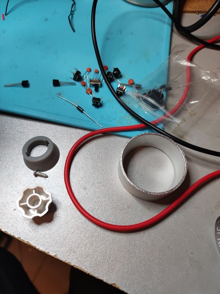
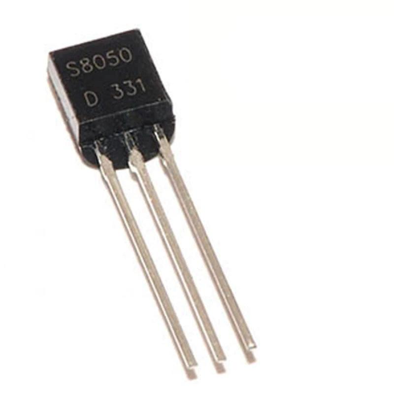
I happened to have NPN transistors available, S8050 specifically (http://media.nkcelectronics.com/datasheet/s8050.pdf)
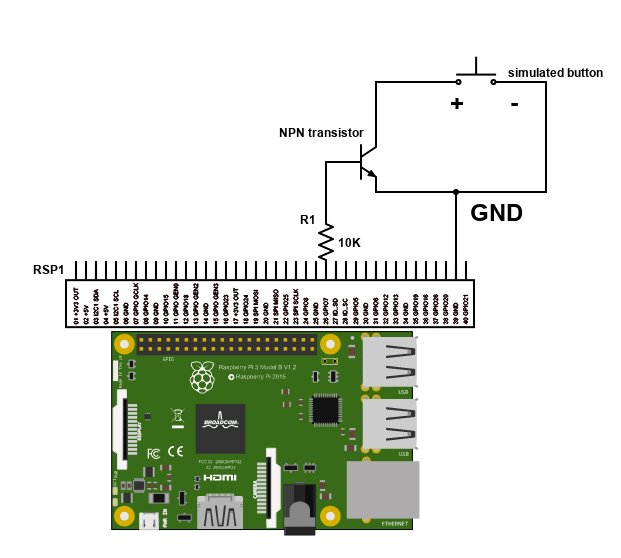
And here is the simple circuit:

I used GPIO 26 here, just make sure you put a 1K to 20K resistor to limit the current on GPIO pin (<10 mA, 3.3V TTL level voltage as a reminder).
« + » voltage of the spray has to be connected to the transistor collector.
« – » side of the spray has to be connected to the common ground (emitter of the transistor).
GPIO has to be programmed as OUTPUT, of course, here is a minimalistic python program to test it:
pi@raspberrypicam:~/soft/gpiotest/mytest $ cat mytest.py
import RPi.GPIO as GPIO
import time
port = 37
GPIO.setmode(GPIO.BOARD)
GPIO.setup(port, GPIO.OUT)
print("high")
GPIO.output(port, GPIO.HIGH)
time.sleep(2)
print("low")
GPIO.output(port, GPIO.LOW)
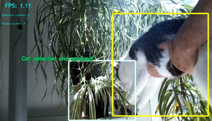
Then the idea is to modify python code from https://github.com/EdjeElectronics/TensorFlow-Object-Detection-on-the-Raspberry-Pi/ to add this spray activation logic!
And some opencv code to add nice text in detection window:


And Now for Something Completely Different, let’s move away from concrete stuff and bite a bit of Machine Learning abstraction (which – who knows – we may plug in a “real life” apparatus) in the good company of indisputably the best story tellers of the 20th century, Carl Barks and Don Rosa.
For the unlucky ones who don’t know them, or rather the lucky ones who don’t know them (who can’t worship them (yet)), Carl Barks and Don Rosa are respectively the creator of the wide Duck world and the guy who refreshed the “franchise”.
They both share a tender respect for the both mild and deep universe they created.
A dive into the awe of an anthropomorphic universe, where adventures always mean discoveries, where gold is often but not always at stake, sometimes Goldie is to be found.

As for Goldie, characters are often not what they appear, Donald Duck despite his uncontrollable anger happens to be the best uncle for his three nephews, most cherished treasures of the stingly Scrooge McDuck are clearly not worth a lot of dollars or the lucky-lookingly Gladstone Glander does not live such a wonderful life, really.
Clearly, that’s an invitation to see characters behind appearances.
Now you may wonder, why such hommage in this blog?
Well, your devoted blog author (myself) being (as you guessed) an idolatrous of this universe, I thought this could be an entertaining opportunity to hands-on Tensorflow, a very accessible neural network framework.
Long term goal is to apply training/inference to real-world devices with sensors, and actuators.
Short term goal, depicted in this article, will be one of the simplest activity offered out-of-the-box by such frameworks (many coexist) : classification.
How? Well, Carl Barks and Don Rosa have very different drawing styles, obvious to the passionate reader.
So I was wondering whether a cold, (a priori) unpassionate convolutional neural net could figure that out.
First, let me restate that this blog is about experiments done out of curiosity, and clearly not written by an expert in the fields and techniques involved.
That being said, your servant (myself) happened to briefly look at the state-of-the-art of neural networks… at the end of last century (the nineties).
A time when perceptrons and Hopfield topologies were ruling keywords under the then-more-restricted neural network realm. A time those under 20 years old cannot know, a more primitive time where sigmoïd were the only viable activation functions, where you had to write your C++ code for your gradient descent (for the learning phase) with your bare p̶a̶l̶m̶s̶ hands.
Good that time is now gone!
So, TensorFlow is a miracle of simplicity exposed to the user compared to that. Plus it has good community, good support among hardware vendors (GPU acceleration via Nvidia Cuda and also A̶T̶I̶ AMD ROCm) but also Google Cloud services (such as the excellent Google Colaboratory, a free environment where you can enjoy dedicated 12 GB with Nvidia Volta GPU or Google’s own TPU).
Will that be enough hardware muscles for only a cold, maybe unpassionate network to perceive the specifics of the two creators? Let’s find out!
Hmm, vast subject.
Your minion (the author of these lines) wrote some lines on that subject back in 2001 in a dedicated website (iacom.fr.st, now redirecting to some unclear Japanese contents).
I would have bet without question that this site has completely vanished into the ashes of the past eternity of the web, but to my great surprise the web archive project kept one copy back in 2013. Only the front page was saved…
Anyway, one of the best short introductions to contemporary n̶e̶u̶r̶a̶l̶ ̶n̶e̶t̶w̶o̶r̶k̶s̶ Deep Learning I can recommend is here: https://codelabs.developers.google.com/codelabs/cloud-tensorflow-mnist
If you can afford more time, I’d recommend the Stanford Coursera course (https://www.coursera.org/learn/machine-learning).
This ellipsis being made, let’s jump into the dataset preparation!
“All quality and no quantity would make our model a dull model.”
Nobody in particular
We have plenty of input data available. Btw, check out the superb volumes edited by Glenat (in France) with lots of annotation/anecdotes, some by Don Rosa himself for the collection dedicated to his work!
In particular if you sometimes fail to discover the hidden D.U.C.K. (Dedicated to Unca Carl from Keno) dedications in the first panels of Don Rosa stories.
I have no doubt that your imagination makes this step unnecessary.
At the end of this stage, we had:
| Stats | |
| Carl Barks, in English | 1158 files 1.35 GB 1.17 MB per file in average |
| Carl Barks, in French | 1544 files 2.8 GB 1.8 MB per file in average |
| Don Rosa, in English | 689 files 0.484 GB 0.702 MB per file in average |
| Don Rosa, in French | 464 files 0.313 GB 0.676 MB per file in average |
Whether we use a stack of only-dense layers (aka old school perceptron) or have mostly convolutional layers, input layer will always have a fixed size, exactly mapping pixel resolution of input images …
This means we have to feed our network during training phase with images of same pixel resolution.


As shown above, terminology related to comics had to be fixed beforehand.
Also, regarding their respective styles, while Carl Barks has a purer, “classic” stroke of pen, Don Rosa, the engineer by training, has definitely profound sense of detail.
While Carl Barks will often sketch everyday life scenes, Don Rosa tends to lean towards epic setups. Naturally, there are many shades of grey in between, these are only tendencies felt by the human reader which I am.

Ideally, in order to compare drawing styles of the two authors, we would feed images with same resolutions.


Both authors created full size images, which could be good samples. However, in case of Carl Barks the intention is more esthetic arts than support for story telling. His drawing style for lithographies is not similar to the one used in his comics. And we want to analyse the style used in the stories.
Also, due to the vast amount of work and time to create such images, there are much less samples falling in these categories.
So we really want to use for our dataset extracts from stories, not these full size images.
Kumiko is an open source tool is a set of tools using OpenCV’s contour detection algorithm to compute meta information on comic pages, such as panels.
A first attempt was done to extract all panels using this tool, but sometimes the algorithm went wrong (borderless panels are difficult to identify). But normalisation would have implied image scaling, and panel shapes are too different to have non destructive shape uniformisation.
So I decided to use images as input of neural networks (knowing that even reduced, such images may not be easy to digest …).
I went for a 1007×648 format, as a compromise between keeping details and not overwhelming our net.
Many pages are descriptive, fully-fletched with text and various layouts.
Also because of Don Rosa’s old engineer habits some pages tend to be … singular ;), such as these very precious ones, depicting Uncle Scrooge’s money bin secret plans:
Useful for the Beagle boys, but clearly not for us.
In order not to interfere with story telling pages, we use Kumiko to count the number of panels.
Kumiko json output
Some Python code helps us to automate the reading-kumiko-panel-meta-information-then-resizing part of input images.
Note, alternatively a rescaling layer can be added at the beginning of our network topology, but that would mean more data to be sent to Colaboratory (as original images are always larger than target resolution).
As can be seen, we only select images for which we detect more than three panels.
Results look good, only meaningful images are left.
However, some visually corrupted images were still present.
Which were easily moved away using, again, simple python logic:
At the end, 1025 clean files remained for Barks/FR, 692 for Barks/EN, 598 for Rosa/EN and 377 for Rosa/FR.
As suggested previously, Google Colaboratory is well integrated into Google’s world. Notably Google Drive.
So after having pushed all files filtered and scaled by our previous python logic (~2.3 GB of .png files compressed in .tar.bz2) to a Google Drive folder, it could be mounted on a Colaboratory session.
After some manual (re)exploration of the dataset, it is time to convert images to Keras input dataset format, and at the same time we want to specify the training/validation ratio.
As we have enough images, we reserve 20% of our sample for the validation:
As we want to train the network to distinguish between Rosa and Barks images, we have two classes, one for each.
The two classes are implicitly detected after the names of the subdirectories from main dataset directories (one class for subdirectory barks/ and the other for rosa/).
Then comes the network topology.
Convulational networks tend to be better then multi dense-layers networks because their cubes-2-cubes internal transformations are somehow better at matching shapes.
Also, that smells newer than our retro perceptrons, so let’s go for it!
Another disclaimer: this experiment was done in a brief amount of time, so no time at all was spend to experiment on various topology variants.
Only the number of neurons in last dense layer was changed a bit.
The rescaling layer at the beginning is just to normalize inputs from 0->255 ranges (RGB colors) to 0->1.
An interesting yet simple explanation for choice of relu activation functions can be read here.

An important thing is to NOT prefetch images in training or validation sets – as it is often the case by default -, otherwise training will quickly cause OOMs (not enough RAM) the session, whatever the batch size is. Because our input images are too big.
After 15 epochs (aka training steps) with batches of 16 images each, we converged to a surprisingly good 99.44% accuracy! 🙂
It took ~22 min to train with a GPU enabled session.
Be careful, by default session starts with no hardware accelerator… so make sure to select it at begining of your session.
Training and accuracy validation plots seem to show 15 epochs should be enough.
However, after attempting some predictions, it appeared another run of 15 epochs did improve results for tested samples.
Despite convergence towards lower accuracy overall:
Interesting is that during 2nd run validation accuracy fell a bit before reincreasing, and redecreasing (could be interesting to test with more epochs). This might be related to overfitting.
First more natural steps would be to stop learning as soon as validation accuracy drops, and training accuracy stops growing (slightly after epoch 15).
As we shuffled both training and validation sets, plus we dedicated a good part to validation (20%), it is not sure massively increasing the amount of training data would help a lot. Decreasing number of model parameters could possibly be key. Or alternatively, we could augment training/validation sets by performing image transformations such as scaling (could help identify full size drawings).
Maybe dropout could be used to reset some neurons at each training iteration. Also, playing with learning rate could be worth testing in a future session.
Funny enough, while reaching a lower accuracy (99.26%), results were much better on samples we used for prediction.
Let’s have a look together at some samples not part of training nor validation set found randomly on the net, and see whether prediction was correct or not (and in parenthesis the confidence factor), and my comments for each picture in legend.


This hands-on on “Deep Learning” was a very fun experiment for me, I really appreciated digging into that.
I’d say results are beyond my initial expectations, however I felt a bit disappointed when the learned model fell in some of the set traps (the “epic” Bark panel for example).
Now, to which extent the model learned the artistic style (whatever this means) or just the layout, the vividness of colorisation or drawing techniques (half a century separates the two!), difficult to say!
However the capability of the model to still have good predictions even for images slightly more exotic than the sometimes rigid 8-panels format used for lots of Carl Barks artworks is appreciable.
Now a next step could be to try other esteemed, modern artists such as Romano Scarpa. Would it still be distinctive enough for a simple model such as the one we trained here?

And who knows, maybe this kind of approach could pave way for artificially generated Duck stories in a not-so-distant future?
Bonjour à toi, puisses tu être fidèle lecteur ou pas.
Un petit post pour partager quelques expérimentations faites à la va-vite quand à l’optimisation des paramètres MultiPath TCP (via l’interface proposée par OpenWRT/OpenMPTCPRouter).
Voici sans tataouiner, comme diraient nos amis québécois, les résultats:
Alors énorme warning, le protocole ne rend en rien honneur à la rigueur forgée par plusieurs siècles de sciences statistiques (pas de calcul de variance par dimension, pas d’estimation d’incertitude).
Ceci dit, on pourra noter qu’en général un seul paramètre est modifié à la fois, avec 3 tests consécutifs par test. Sauf exception, auquel cas on se retrouve dans une configuration déjà testée (ou.. presque).
Les tests ont été fait de façon groupée, avec des conditions météos similaires (important, car nous parlons d’interfaces 4G).
On force pour tous les runs le serveur speedtest auquel une CLI se connecte pour mesure.
Si l’on souhaite creuser la signification de quelques paramètres MPTCP, il y a la Source (http://multipath-tcp.org/, par les auteurs contribuant dans le noyau Linux, malheureusement pas tout à fait à jour), ainsi que de nombreux blogs/publications que l’on peut dénicher sur le net (http://staff.ustc.edu.cn/~kpxue/paper/Sigcomm2019-p75-Han.pdf, https://www.gitmemory.com/marcschaller, https://hal.sorbonne-universite.fr/hal-01382907v2/document), dont les résultats ont parfois permis de limiter le champs d’exploration pour nos petites expériences (notamment pour la combinatoire des “congestion protocol”, avec certains comme balia, olia ou encore wvegas clairement en retrait dans le cadre de ma double connexion 4g).
Un point intéressant, on pourrait très clairement envisager l’utilisation pertinente (pour une fois 😉 ) d’apprentissage supervisé (reinforcement learning par exemple) pour parcourir de manière non exhaustive la combinatoire, et de converger vers un objectif à définir.
Dans mon cas (multiplexage de connexions internet 4g pour télétravailler, essentiellement), l’objectif est de minimiser la gigue (aka jitter en anglais) et le ping, pour rendre le plus agréable possible les appels audio et vidéoconférences.
Ensuite, il s’agit de minimiser les pertes de paquets pour éviter de subites pertes de connections SSH ou VPN, par exemple.
Enfin, avec une moindre priorité, de maximer la bande passante en téléchargement (download et upload).
Le scheduler “redundant” est à éviter, il provoque un débit quasiment deux fois moindre que ses meilleurs comparses.
Même sentence pour le pathmanager “binder”, il est le seul à être accompagné de systématiques pertes de paquets.
Il serait intéressant de creuser l’impact du nombre de “subflows” par couple d’ip source/destination, même si l’asymptote semble vite atteinte.

était le combo:
path manager: fullmesh
scheduler: ECF (a priori meilleur pour les liens « aériens » comme la 4G)
congestion control: mtcpdesync
avec 2 subflow par pair d’IPs.
Les défauts étant resp. fullmesh/BLEST/cubic.
Depuis l’écriture originelle de cet article et l’incendie d’OVH qui a obligé une réécriture (rapide, il faut dire) des derniers articles de ce blog, j’ai découvert qu’après quelques heures, cette configuration mettait le VPS à genoux.
Après quelques itérations, en remettant la valeur par défaut au paramètre “fullmesh subflows for each pair of IP addresses”, soit 1, le retour à la stabilité était atteint.
D’autres itérations restaient toutefois nécessaires. En particulier, comprendre d’ou venait l’effondrement en performance (empreinte cpu/mémoire lié aux subflows, effet collatéral lié à du swap (si starvation mémoire..)..?).
Les derniers essais fait sur un autre fournisseur VPS, avec 2 Go de RAM (plutot qu’un seul), ainsi que l’arrivée d’un nouvel algorithme de contrôle de congestion (bbr2 en beta), indique désormais le combo ECF/bbr2 en combo gagnant.
Avec les paramètres par défaut:
Voici les résultats:
Et avec le combo ECF/bbr2:
Des résultats excellents!
Note, le passage a 2 fullmesh subflows par paire d’IPs ne semble avoir aucun impact avec le nouveau VPS (2 vCores Intel Xeon E5-2690v3 + 2Go ram), alors au vu de l’impact sur le VPS précédent, j’ai décidé d’en rester à la valeur par défaut.
Note 2, les IPs des VPS OVH étant blacklistés par de nombreux sites/services (blink d’Amazon par exemple), le passage au nouveau VPS (pulseheberg) évite le paramétrage omr-bypass, qui permet de garder l’intérêt de la solution en toutes circonstances.
Note: l’article originale était illustrée de moults images, photos mais suite à la destruction du datacentre d’OVH de mars 2021 (ou ce blog était hosté, les images ont été perdues, seul le texte des articles a pu être sauvé)
Alors, ceci se veut le résumé d’une très longue histoire, celle de la quête d’une connexion “acceptable” dans l’arrière pays du Sud de la France.
Après avoir trouvé la maison de nos rêves (mi 2019), maison qui coche un maximum de cases, un compromis a cependant du être trouvé quand à la connectivité vers l’internet mondial, si utile par ces temps.
Au point initial, nous avons:
Parlons en, des services de test de débit à partir de l’ancien numéro de téléphone et/ou adresse postale.
Dans notre cas, nous avions 30 Mb/s via degrouptest.com, mais les autres (ariase, ovh..) sont d’accord.
ok, pas si terrible que ça que vous me direz!
Après abonnement sosh, nous plafonnons à 2.1 Mb/s, le vent dans le dos.
Soit 260 ko/s. En 2020, ça fait un peu tache. Surtout pour télétravailler..
Et en 3G, nous plafonnions à 8 Mb/s. Mieux, mais pas terrible..
Sans rentrer dans les détails, une visite dans le NRA en question a permis de résoudre ce mystère.
En effet, le NRA était bien à moins de 900 mètres du domicile, et non, pas de souci de condensateurs ou autres défauts augmentant l’atténuation du signal.
Le souci venait de la nature du signal arrivant au NRA. En France, il semble que la plupart des NRA/NRO sont inter-reliés par des réseaux de fibre optique. Ce qui semble être l’hypothèse de (tous?) les services de test de débit, le goulot d’étranglement étant alors la distribution entre le NRA et l’abonné.
Mais non, certains NRA sont inter-reliés par des faisceaux hertziens propriétaires (autour de 1 Ghz). Dans ce cas, le débit total par NRA tourne autour de quelques centaines de Mbits/s, débit partagé par les centaines de lignes analogiques physiquement raccordées.
D’où un débit bridé à ~2Mbit/s par abonné dans ces situations.
Déjà, nous pouvions abandonner la ligne terrestre.
Restaient:
La piste à creuser apparaissait alors évidente.
Pour cela, j’ai commencé avec ce site: www.monreseaumobile.fr
Mais j’ai été déçu par les données non actualisées, très peu précises (notamment sur le type et la position des antennes) et des estimations de “qualité” du signal fantaisistes (dans l’arrière pays, du moins).
Ce qui n’était pas le cas de ce site: www.antennesmobiles.fr
Il suffit de sélectionner les antennes type 4G (et 5G si vous êtes rêveurs), et de vous trouver en vous aidant de la géolocalisation (code postal par exemple).
www.cartoradio.fr est également très pratique, car il indique également les orientations des antennes (aussi appelées azimuts).
Par la suite, difficile de montrer une procédure précise sans dévoiler la localisation de votre serviteur-auteur de cet article.
www.cartoradio.fr, information que l’on peut croiser avec celles d’antennesmobiles.fr (avec l’ID)
Ici on voit l’azimut
On a une information plus ou moins précise, c’est variable, de la localisation/adresse de l’antenne.
Ensuite, autre outil indispensable: https://www.geoportail.gouv.fr/carte
Il suffit de prendre le fond de carte “carte du relief”, puis en mode 2D
Puis d’annoter votre maison, et les différentes antennes localisées grâce à leur adresse, ou alors si besoin en s’aidant du calque “Plan IGN” de geoportail:
Et là, la vue permet de facilement identifier:
Pour ce dernier point, on peut aussi s’aider de l’outil de calcul du profil altimétrique.
On peut tracer une ligne droite sur le profil, pour bien voir ou se trouvent les obstacles
Et dans ce cas on voit que cela ne passerait pas.
A comparer avec les orientations fournies par cartoradio.
Il suffit de jouer un peu, en considérant aussi d’autres paramètres, comme les fréquences auxquelles on peut être candidat.
Une fréquence basse (700 Mhz, 800 Mhz) sera plus “passe partout”, car moins sensible à un air chargé en humidité, ou quand il pleut.
Une fréquence haute sera, si captée avec un bon ratio signal/bruit, synonyme d’un meilleur débit.
Aussi, il sera utile de repérer la densité en habitant autour ces antennes (présences de villages, villes, combien d’habitants..), et imaginer un “iso-signal” (c’est à dire voir les zones qui sont le mieux desservies par les antennes repérées, plutôt peuplées ou non) pour éviter les antennes trop fréquentées.
Après l’étape 1, tu sauras cher lecteur quelle est ou quelles sont les fréquences avec lesquelles tu vas travailler.
Fort de ces informations, tu trouveras utile ou non de t’orienter sur un routeur à aggrégation de porteuses (attention, si l’opérateur propose lui même 1) plusieurs bandes de fréquences sur l’antenne considérée et 2) s’il propose l’aggrégation de fréquences), aussi appelée 4G+ (800 Mhz + 1800 Mhz chez Bouygues, 800 Mhz + 2600 Mhz chez Bouygues, Orange, SFR, ou 1800 Mhz + 2600 Mhz chez Bouygues ou Free) ou 4G++ (3 bandes de fréquence).
Pour les détails sur le hardware qui va bien, je t’invite à regarder ce site: https://routeur4g.fr/
J’ai pour la part jeté mon dévolu sur cette antenne (très efficace, un peu chère) et celle ci (sensiblement moins efficace, moins chère).
Branchées respectivement sur un routeur 4g Huawei B715 et une clé 4G E3372h-607.
Il suffit de suivre les “bons plans” sur les forfait 4g.
Dans notre optimisation, nous avons un forfait crédit mutuel mobile à 25 euros/mois avec “data illimitée” (en vrai 2000 GO/mois) et une deuxième carte sim greffée à un forfait Bouygues (option facturée 2 euros/mois).
Edit: On m’a signalé que le forfait c’redit mutuel mobile n’est plus dispo au même tarif. Je recommande de surveiller les bons plans en la matière, qui reviennent régulièrement.
Il faut être stratégique sur l’assignation de l’abonnement au forfait.
Le forfait le plus gros, sur le couple routeur/antenne le plus performant (car il se videra plus vite).
Le lecteur intéressé, facétieux et attentif que tu es aura remarqué que l’auteur de ce post fait référence plusieurs fois à deux moyens d’accès à Internet.
Il existe des routeurs wifi qui permettent une aggrégation de façon plus ou moins native (par ex, un asus RT-3200 sert ton serviteur, qui propose un link aggregation).
Mais en vrai, ça ne marche pas bien.
Car c’est soit une aggrégation de connections TCP – qui permet de maximiser la bande passante uniquement dans certains cas “faciles” (protocoles nativement multiconnections comme torrent), ou alors du fail over (si un lien tombe, l’autre est utilisé, ce qui revient à bien cher pour cet usage uniquement).
Il existe quelques rares options commerciales, comme overthebox, qui permettent une aggrégation plus basse, au niveau TCP.
Mais les tarifs autrefois abordables ne le sont plus (150 euros HT de boitier + 20 euros HT, au moins cher, avec 100 Mb/s max en aggrégation.
Mais une alternative peu dispendieuse existe désormais, https://www.openmptcprouter.com/
L’idée:
votre réseau local est physiquement branché sur un raspberry (d’autres hardwares supportés, mais moins bien), sur lequel une distribution OpenWrt customisée est installée, et connecté via VPN à un serveur disposant d’une IP publique, et préférablement d’une bande passante confortable. Un VPS est un excellent choix.
Je recommanderais un VPS OVH (à partir de 3 euros TTC/mois), mais l’offre est pléthorique.
Comme votre dévoué fabidouille avait déjà un VPS (pour hoster ce site notamment), le coût de l’opération s’avérait minime.
Un bon résumé des avantages de cette approche est disponible sur Wikipedia.
La redondance offerte par Multipath TCP rend accessible le multiplexage inverse de ressources, ce qui permet d’améliorer la cadence (throughput) de TCP jusqu’à atteindre la somme des cadences en profitant des performances des différents canaux physiques au lieu de n’en utiliser qu’un seul, comme c’est le cas en TCP standard. Multipath TCP est en plus rétro-compatible avec le TCP classique.
Pour l’installation de la partie serveur, ça se passe ici.
Et pour la partie client (raspberry), ça se passe là.
Autre immense avantage, la possibilité de plus avoir son adresse IP NATée, ce qui serait le cas en 4G classique.
Pour le dire simplement, pour économiser le nombre d’IPs v4 attribuées aux clients 4G, une adresse publique est partagée par de multiples utilisateurs, via un réseau NAT. Ce qui rend l’exposition de service impossible, sans tiers partie.
Mais cette approche permet de profiter de l’adresse IP v4 statique (ainsi que les noms de domaines associés éventuellement) à son VPS, ainsi que d’autres avantages (par ex protection DDOS OVH).
Si ton sens de l’économie est assez aiguisé, tu souhaiteras peut être utiliser ton serveur VPS pour héberger un site, un accès https domotique, des accès à d’autres services exposés sécurisés, ainsi que des services non exposés internes (comme DNS avec Pi-Hole).
Dans ce cas, il faut faire attention à
Au final, un petit schéma (simplificateur 😉 – on ne montre pas toutes les interfaces réseaux côté client/VPS) pour ne pas trop s’y perdre
Du fait de quelques instabilités et surtout un peu de gigue (variations qui pouvait être importantes dans l’étalement, la “périodicité” des paquets TCP), l’utilisation du scheduler “redundant” (plutôt que BLEST) donne de bons résultats pour le moment.
Quelques infos intéressantes ici sur l’implémentation de ce scheduler, issue d’un projet de l’Union Européenne en sécurité: https://github.com/i2t/rmptcp
Aujourd’hui, un petit déballage sur un achat fait sur gearbest deux ans après l’achat, un prometteur objet titré “Utorch LED Mosquito Killer Lighting Bulb – White 220V”.
Alors obtenu contre 5.22 euros, j’ai eu une triple surprise en le recherchant alors que j’écris ce billet.
Si on met de côté le régal que des traductions de ce genre d’article, on voit les logos CE (pour Chinese Export » 😉 ?) et Interdit aux petits oignons dans une tente (ou.. non dimmable).
qui nous rassurent d’emblée.
Déjà, à peine la boite ouverte, deux morceaux en tombent.
Un couvercle en plastique et le corps de l’ampoule.
Et oui, les deux parties n’étaient pas solidaires en sortie de boite.
Wahou!
En fausses couleurs, pour augmenter le contraste, on comprends un peu mieux le schéma. A analyser dans le détail, mais il semblerait que la conversion AC->DC se fasse par un simple pont de diode (M310F), sans séparation primaire/secondaire par transfo.
Voilà, le quickie est déjà terminé.
Qu’en déduire? Au minimum couper les bouts de fil pour limiter les risques de court circuit, et éviter de la laisser dehors sans protection..