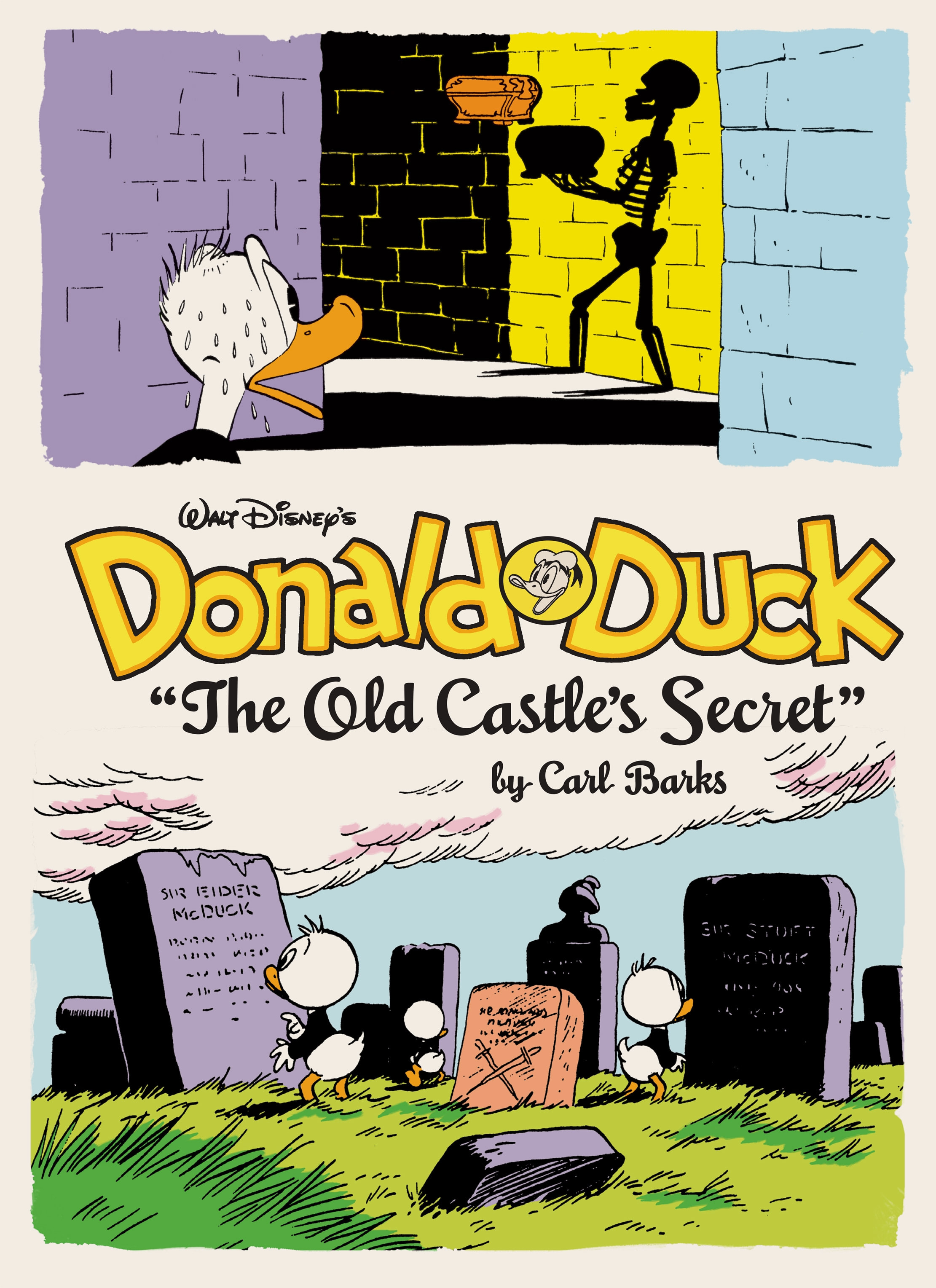
And Now for Something Completely Different, let’s move away from concrete stuff and bite a bit of Machine Learning abstraction (which – who knows – we may plug in a “real life” apparatus) in the good company of indisputably the best story tellers of the 20th century, Carl Barks and Don Rosa.
The Masters of a rich palmed world
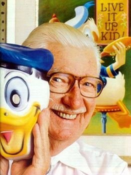
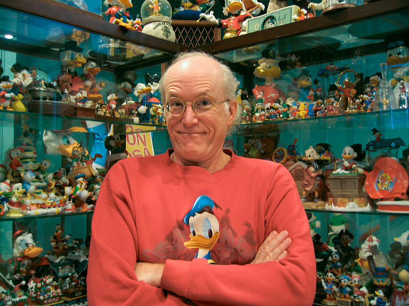
For the unlucky ones who don’t know them, or rather the lucky ones who don’t know them (who can’t worship them (yet)), Carl Barks and Don Rosa are respectively the creator of the wide Duck world and the guy who refreshed the “franchise”.
They both share a tender respect for the both mild and deep universe they created.
A dive into the awe of an anthropomorphic universe, where adventures always mean discoveries, where gold is often but not always at stake, sometimes Goldie is to be found.
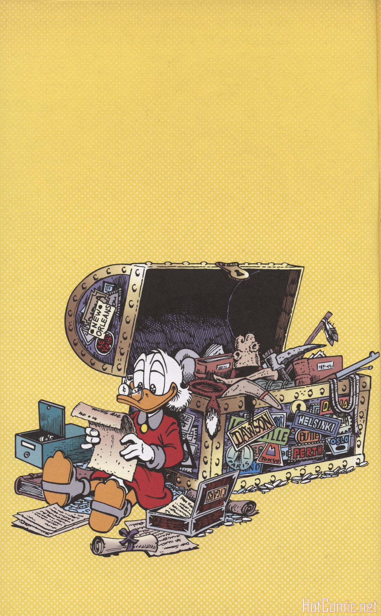
As for Goldie, characters are often not what they appear, Donald Duck despite his uncontrollable anger happens to be the best uncle for his three nephews, most cherished treasures of the stingly Scrooge McDuck are clearly not worth a lot of dollars or the lucky-lookingly Gladstone Glander does not live such a wonderful life, really.
Clearly, that’s an invitation to see characters behind appearances.
Ok, then what?
Now you may wonder, why such hommage in this blog?
Well, your devoted blog author (myself) being (as you guessed) an idolatrous of this universe, I thought this could be an entertaining opportunity to hands-on Tensorflow, a very accessible neural network framework.
Long term goal is to apply training/inference to real-world devices with sensors, and actuators.
Short term goal, depicted in this article, will be one of the simplest activity offered out-of-the-box by such frameworks (many coexist) : classification.
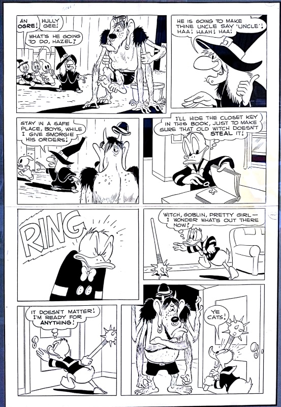
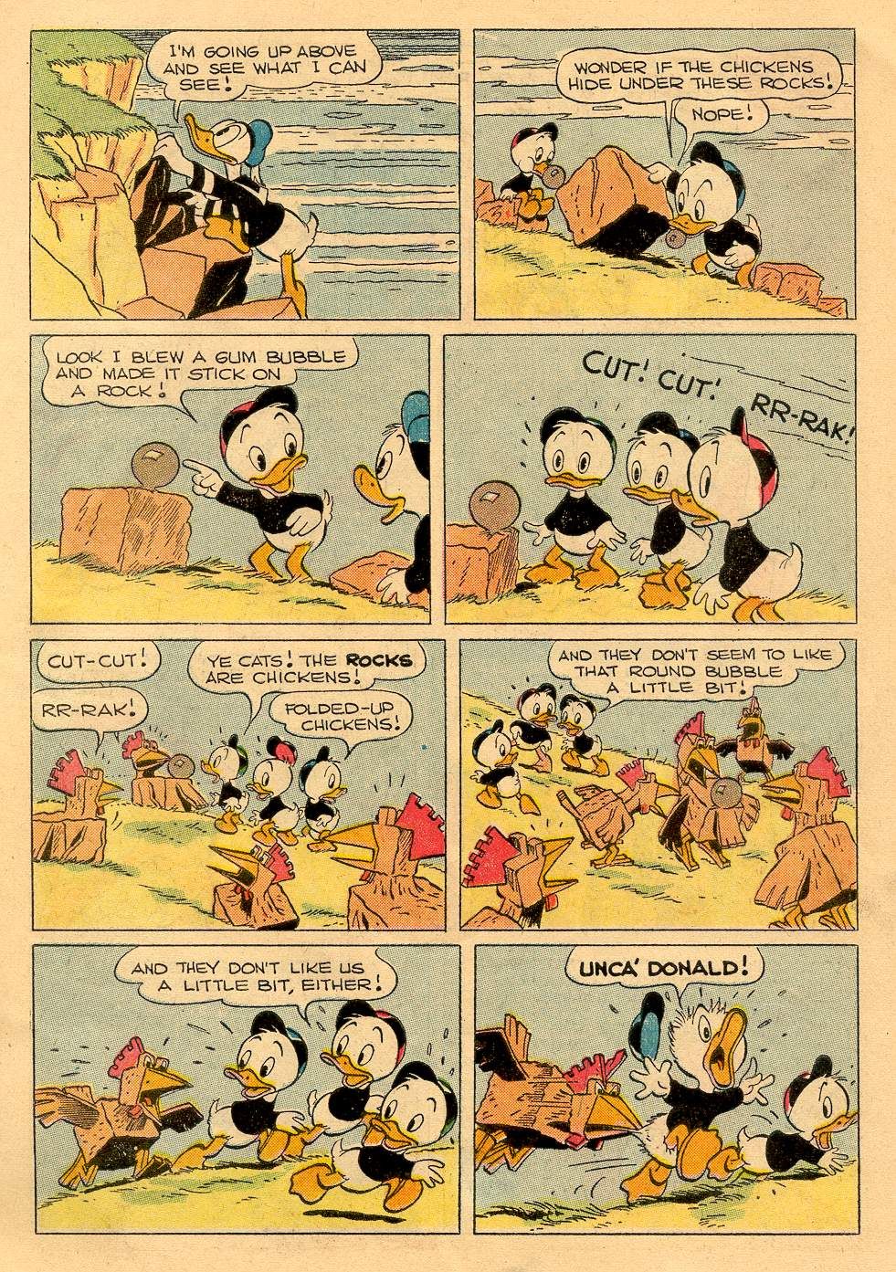
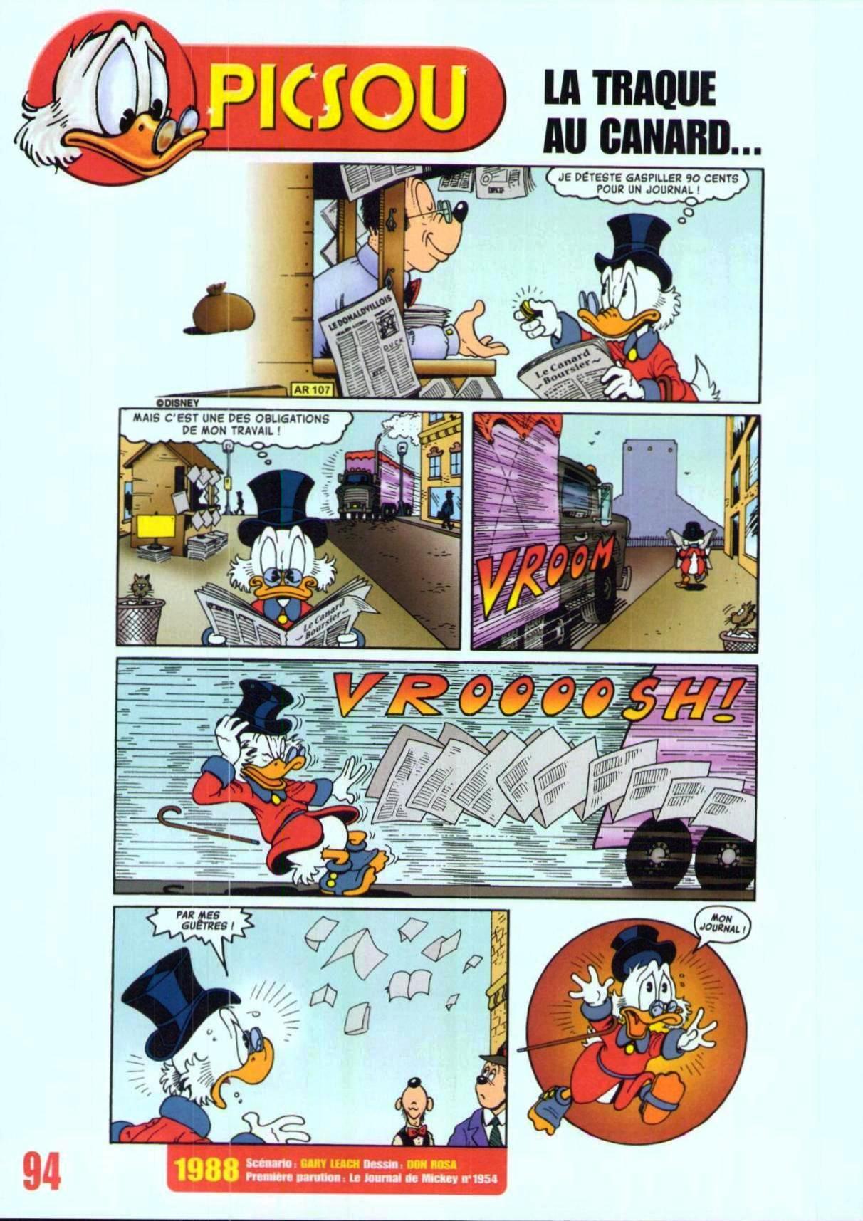
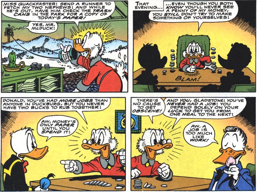
How? Well, Carl Barks and Don Rosa have very different drawing styles, obvious to the passionate reader.
So I was wondering whether a cold, (a priori) unpassionate convolutional neural net could figure that out.
Why Tensorflow?
First, let me restate that this blog is about experiments done out of curiosity, and clearly not written by an expert in the fields and techniques involved.
That being said, your servant (myself) happened to briefly look at the state-of-the-art of neural networks… at the end of last century (the nineties).
A time when perceptrons and Hopfield topologies were ruling keywords under the then-more-restricted neural network realm. A time those under 20 years old cannot know, a more primitive time where sigmoïd were the only viable activation functions, where you had to write your C++ code for your gradient descent (for the learning phase) with your bare p̶a̶l̶m̶s̶ hands.
Good that time is now gone!
So, TensorFlow is a miracle of simplicity exposed to the user compared to that. Plus it has good community, good support among hardware vendors (GPU acceleration via Nvidia Cuda and also A̶T̶I̶ AMD ROCm) but also Google Cloud services (such as the excellent Google Colaboratory, a free environment where you can enjoy dedicated 12 GB with Nvidia Volta GPU or Google’s own TPU).
Will that be enough hardware muscles for only a cold, maybe unpassionate network to perceive the specifics of the two creators? Let’s find out!
By the way, what is a neural network, and how could it classify drawings?
Hmm, vast subject.
Your minion (the author of these lines) wrote some lines on that subject back in 2001 in a dedicated website (iacom.fr.st, now redirecting to some unclear Japanese contents).
I would have bet without question that this site has completely vanished into the ashes of the past eternity of the web, but to my great surprise the web archive project kept one copy back in 2013. Only the front page was saved…
Anyway, one of the best short introductions to contemporary n̶e̶u̶r̶a̶l̶ ̶n̶e̶t̶w̶o̶r̶k̶s̶ Deep Learning I can recommend is here: https://codelabs.developers.google.com/codelabs/cloud-tensorflow-mnist
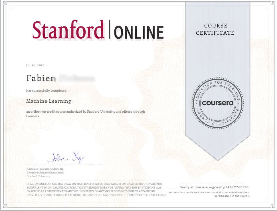
If you can afford more time, I’d recommend the Stanford Coursera course (https://www.coursera.org/learn/machine-learning).
This ellipsis being made, let’s jump into the dataset preparation!
Dataset preparation
“All quality and no quantity would make our model a dull model.”
Nobody in particular
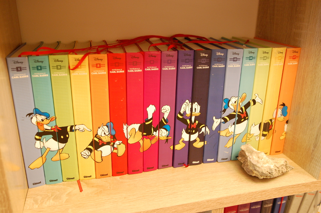
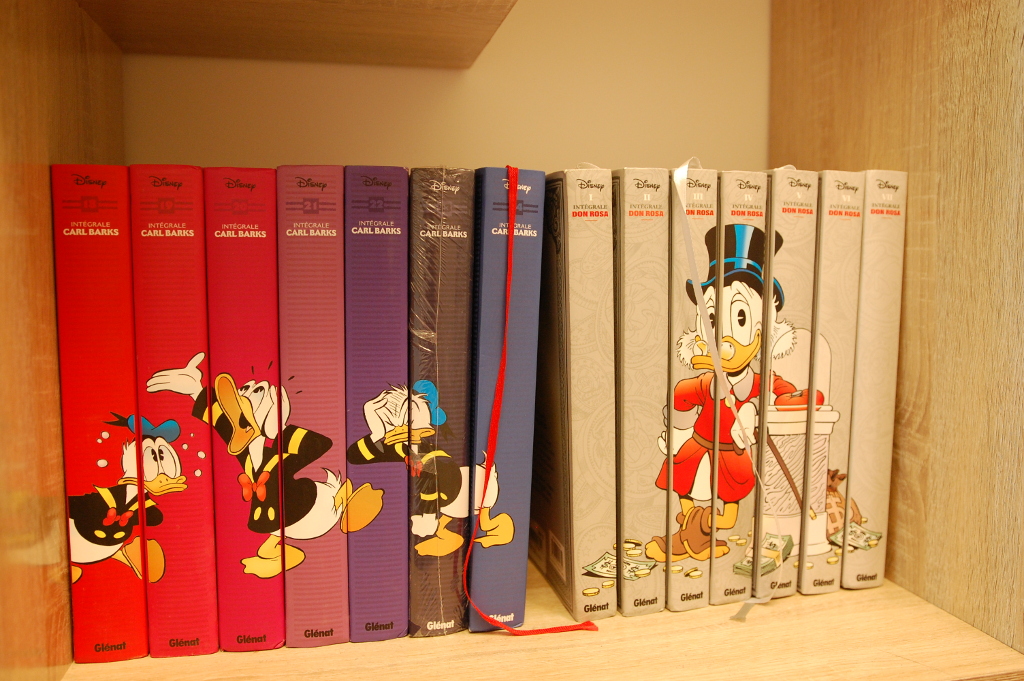
We have plenty of input data available. Btw, check out the superb volumes edited by Glenat (in France) with lots of annotation/anecdotes, some by Don Rosa himself for the collection dedicated to his work!
In particular if you sometimes fail to discover the hidden D.U.C.K. (Dedicated to Unca Carl from Keno) dedications in the first panels of Don Rosa stories.
Digitization
I have no doubt that your imagination makes this step unnecessary.
At the end of this stage, we had:
| Stats | |
| Carl Barks, in English | 1158 files 1.35 GB 1.17 MB per file in average |
| Carl Barks, in French | 1544 files 2.8 GB 1.8 MB per file in average |
| Don Rosa, in English | 689 files 0.484 GB 0.702 MB per file in average |
| Don Rosa, in French | 464 files 0.313 GB 0.676 MB per file in average |
Filtering
Whether we use a stack of only-dense layers (aka old school perceptron) or have mostly convolutional layers, input layer will always have a fixed size, exactly mapping pixel resolution of input images …
This means we have to feed our network during training phase with images of same pixel resolution.

As shown above, terminology related to comics had to be fixed beforehand.
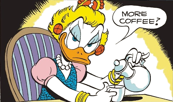
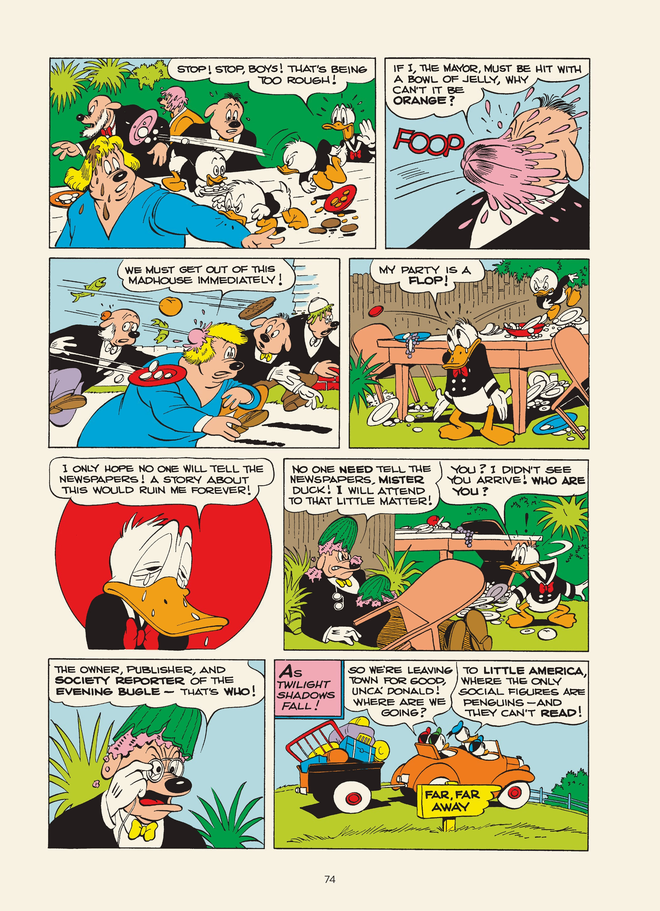
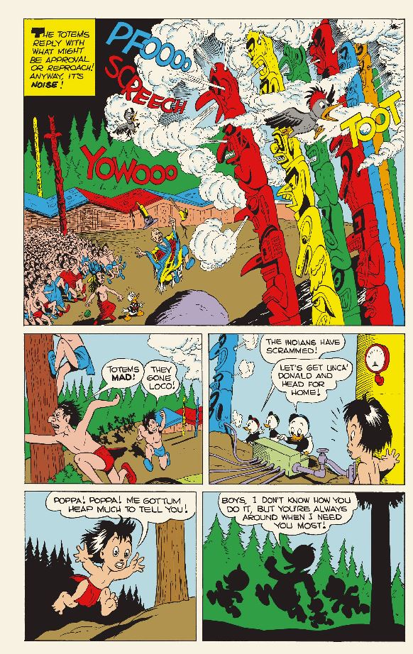
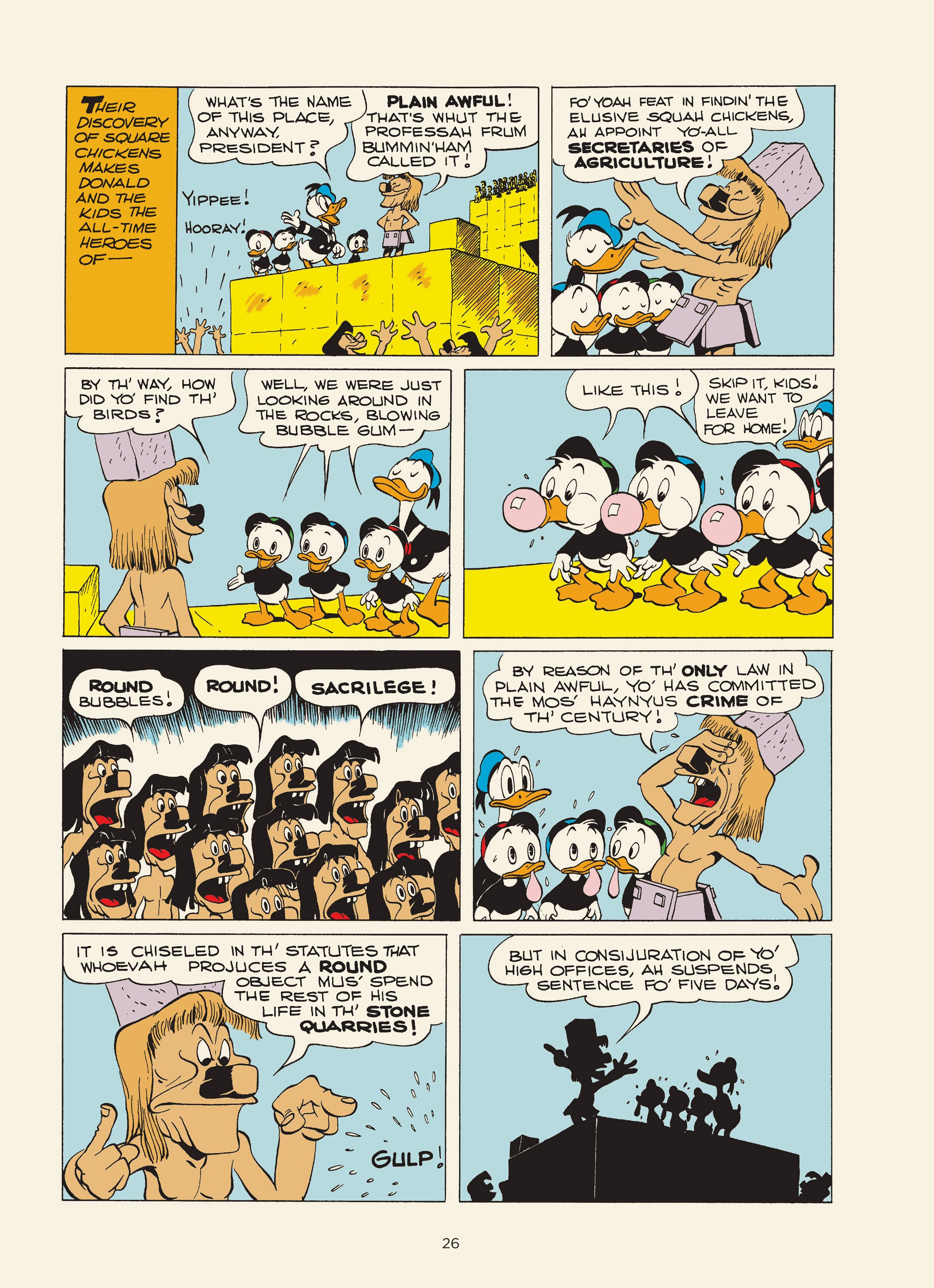
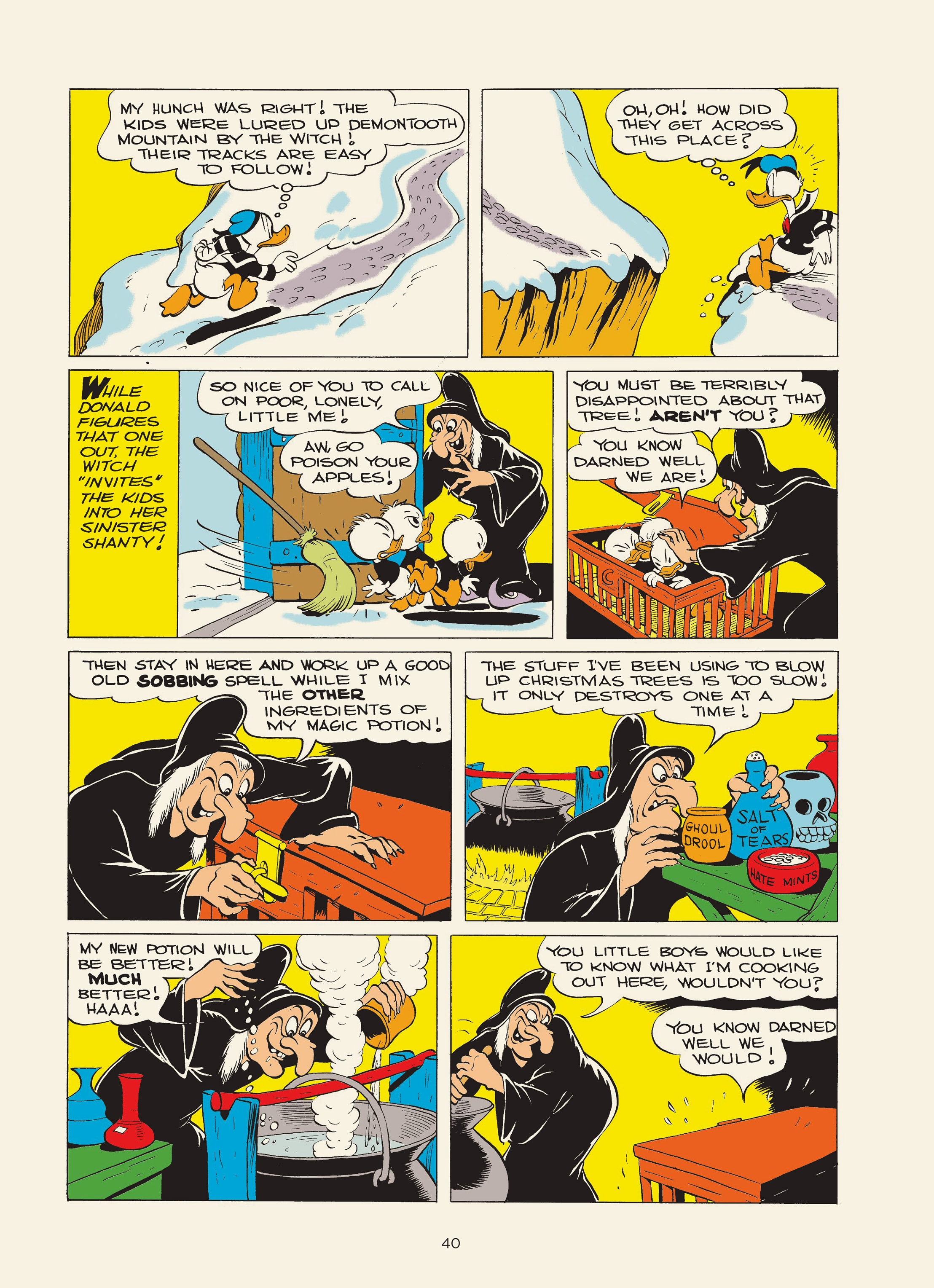
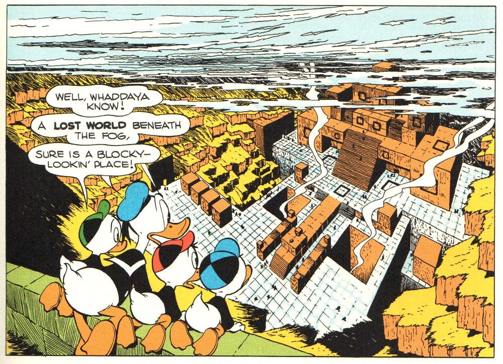
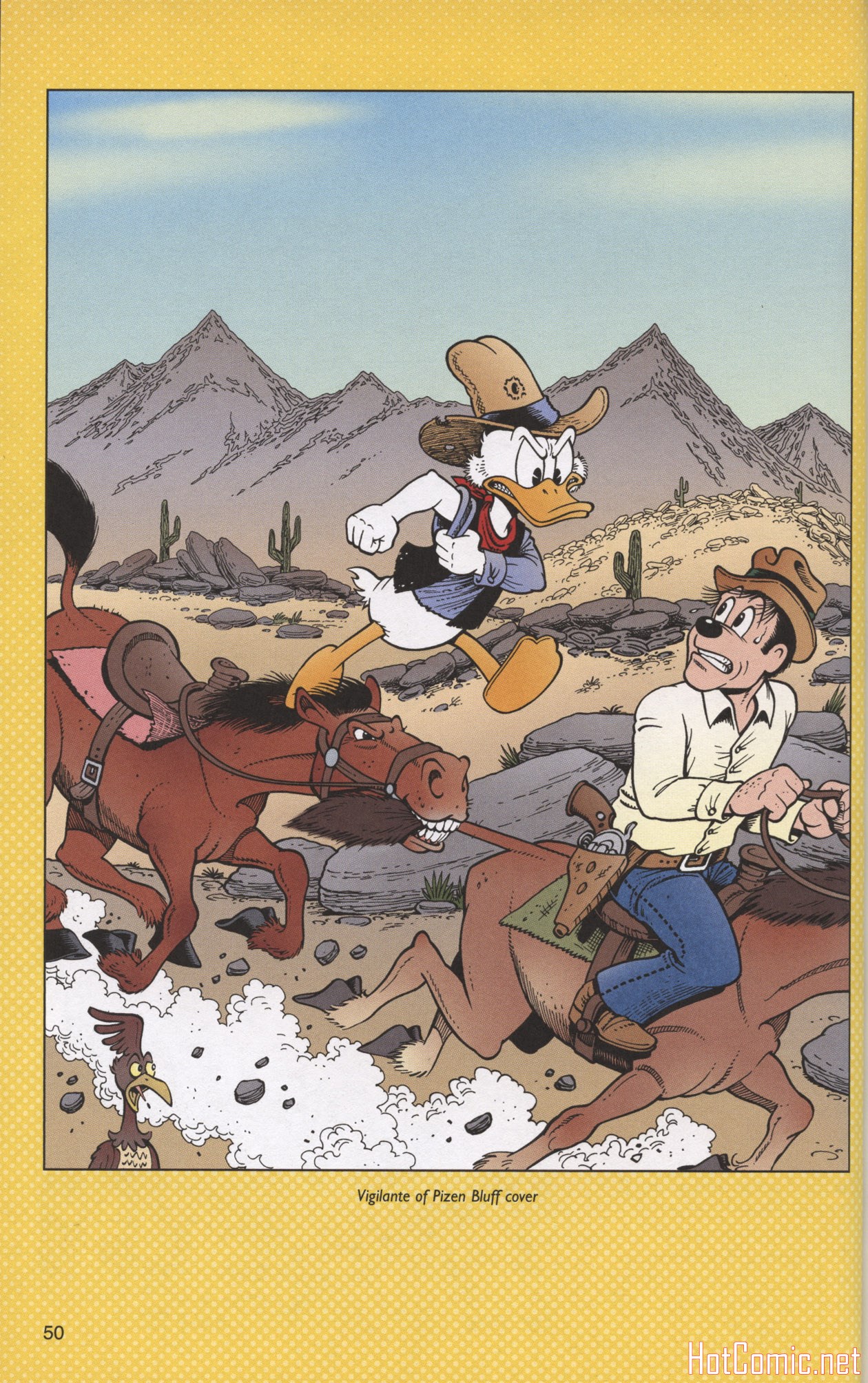
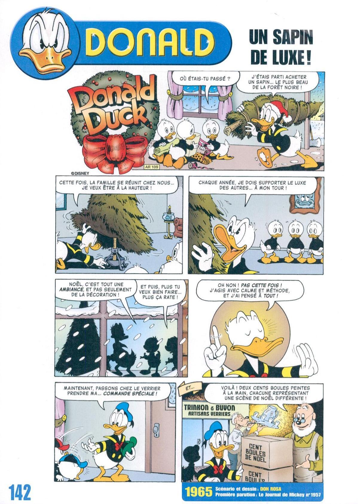
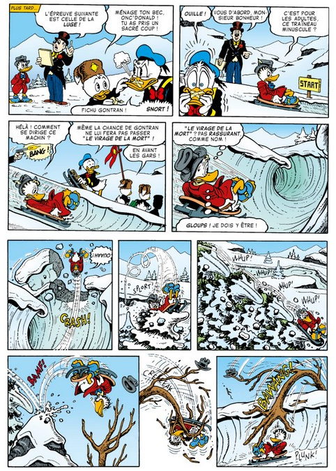
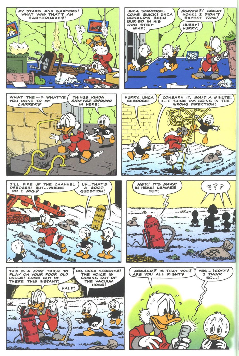
Also, regarding their respective styles, while Carl Barks has a purer, “classic” stroke of pen, Don Rosa, the engineer by training, has definitely profound sense of detail.
While Carl Barks will often sketch everyday life scenes, Don Rosa tends to lean towards epic setups. Naturally, there are many shades of grey in between, these are only tendencies felt by the human reader which I am.
Ideally, in order to compare drawing styles of the two authors, we would feed images with same resolutions.
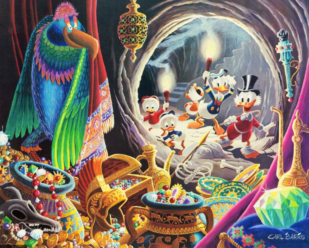
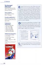
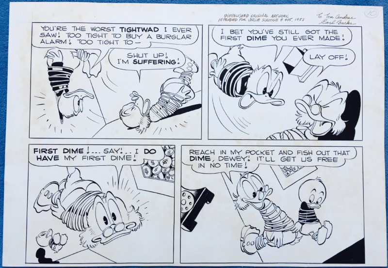
Both authors created full size images, which could be good samples. However, in case of Carl Barks the intention is more esthetic arts than support for story telling. His drawing style for lithographies is not similar to the one used in his comics. And we want to analyse the style used in the stories.
Also, due to the vast amount of work and time to create such images, there are much less samples falling in these categories.
So we really want to use for our dataset extracts from stories, not these full size images.
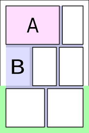
Page panel extraction : Kumiko
Kumiko is an open source tool is a set of tools using OpenCV’s contour detection algorithm to compute meta information on comic pages, such as panels.
A first attempt was done to extract all panels using this tool, but sometimes the algorithm went wrong (borderless panels are difficult to identify). But normalisation would have implied image scaling, and panel shapes are too different to have non destructive shape uniformisation.
So I decided to use images as input of neural networks (knowing that even reduced, such images may not be easy to digest …).
I went for a 1007×648 format, as a compromise between keeping details and not overwhelming our net.
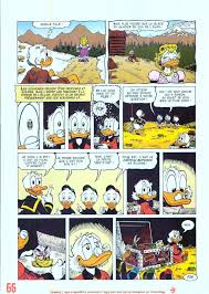
Many pages are descriptive, fully-fletched with text and various layouts.
Also because of Don Rosa’s old engineer habits some pages tend to be … singular ;), such as these very precious ones, depicting Uncle Scrooge’s money bin secret plans:
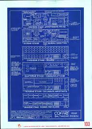
Useful for the Beagle boys, but clearly not for us.
In order not to interfere with story telling pages, we use Kumiko to count the number of panels.
Kumiko json output
![]()
Some Python code helps us to automate the reading-kumiko-panel-meta-information-then-resizing part of input images.
Note, alternatively a rescaling layer can be added at the beginning of our network topology, but that would mean more data to be sent to Colaboratory (as original images are always larger than target resolution).
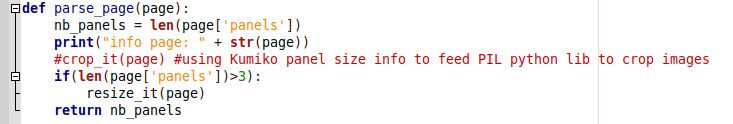
As can be seen, we only select images for which we detect more than three panels.
Results look good, only meaningful images are left.
However, some visually corrupted images were still present.

Which were easily moved away using, again, simple python logic:
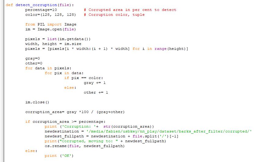
At the end, 1025 clean files remained for Barks/FR, 692 for Barks/EN, 598 for Rosa/EN and 377 for Rosa/FR.
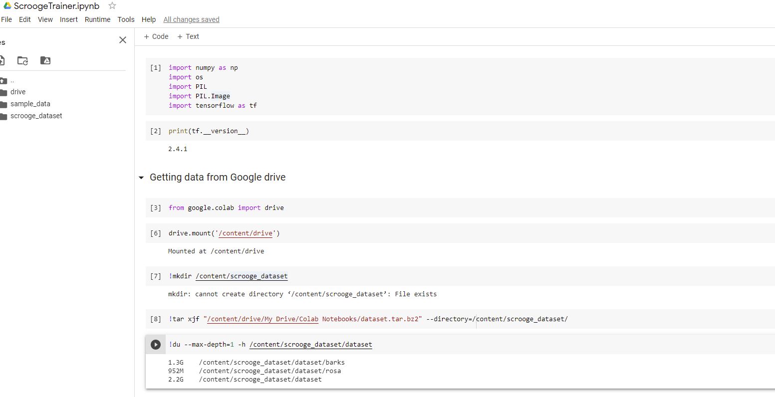
Now, let’s get into Tensorflow!
As suggested previously, Google Colaboratory is well integrated into Google’s world. Notably Google Drive.
So after having pushed all files filtered and scaled by our previous python logic (~2.3 GB of .png files compressed in .tar.bz2) to a Google Drive folder, it could be mounted on a Colaboratory session.
After some manual (re)exploration of the dataset, it is time to convert images to Keras input dataset format, and at the same time we want to specify the training/validation ratio.
As we have enough images, we reserve 20% of our sample for the validation:
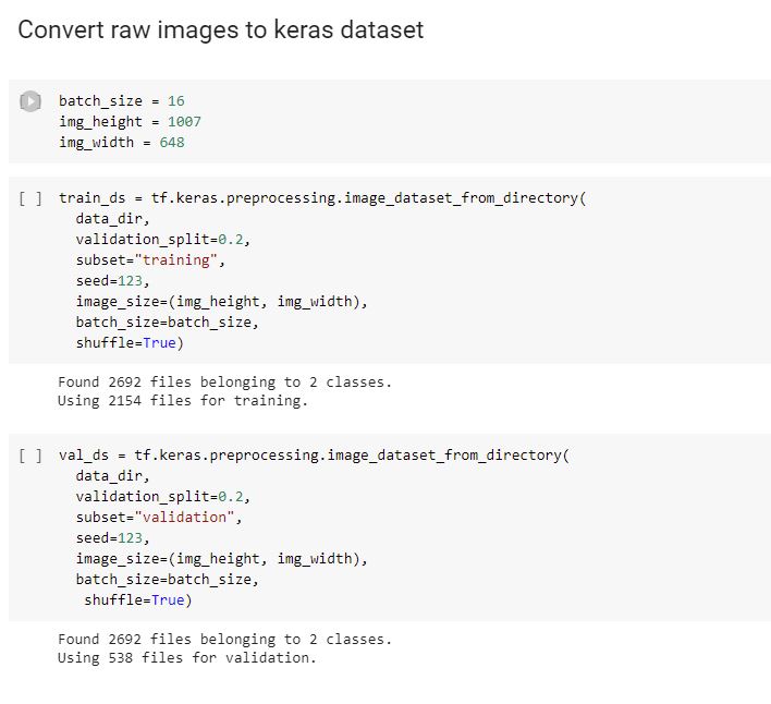
As we want to train the network to distinguish between Rosa and Barks images, we have two classes, one for each.
The two classes are implicitly detected after the names of the subdirectories from main dataset directories (one class for subdirectory barks/ and the other for rosa/).
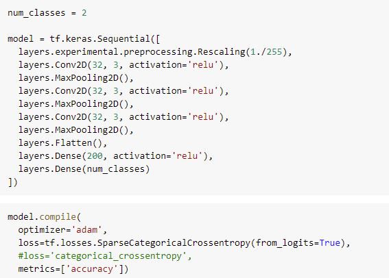
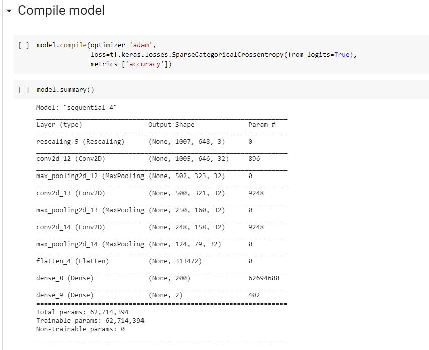
Then comes the network topology.
Convulational networks tend to be better then multi dense-layers networks because their cubes-2-cubes internal transformations are somehow better at matching shapes.
Also, that smells newer than our retro perceptrons, so let’s go for it!
Another disclaimer: this experiment was done in a brief amount of time, so no time at all was spend to experiment on various topology variants.
Only the number of neurons in last dense layer was changed a bit.
The rescaling layer at the beginning is just to normalize inputs from 0->255 ranges (RGB colors) to 0->1.
An interesting yet simple explanation for choice of relu activation functions can be read here.
An important thing is to NOT prefetch images in training or validation sets – as it is often the case by default -, otherwise training will quickly cause OOMs (not enough RAM) the session, whatever the batch size is. Because our input images are too big.
After 15 epochs (aka training steps) with batches of 16 images each, we converged to a surprisingly good 99.44% accuracy! 🙂
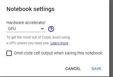
It took ~22 min to train with a GPU enabled session.
Be careful, by default session starts with no hardware accelerator… so make sure to select it at begining of your session.
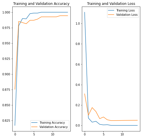
Training and accuracy validation plots seem to show 15 epochs should be enough.
However, after attempting some predictions, it appeared another run of 15 epochs did improve results for tested samples.
Despite convergence towards lower accuracy overall:
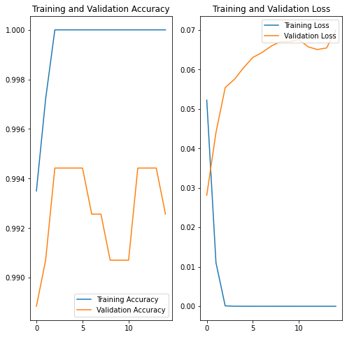
Interesting is that during 2nd run validation accuracy fell a bit before reincreasing, and redecreasing (could be interesting to test with more epochs). This might be related to overfitting.
First more natural steps would be to stop learning as soon as validation accuracy drops, and training accuracy stops growing (slightly after epoch 15).
As we shuffled both training and validation sets, plus we dedicated a good part to validation (20%), it is not sure massively increasing the amount of training data would help a lot. Decreasing number of model parameters could possibly be key. Or alternatively, we could augment training/validation sets by performing image transformations such as scaling (could help identify full size drawings).
Maybe dropout could be used to reset some neurons at each training iteration. Also, playing with learning rate could be worth testing in a future session.
Funny enough, while reaching a lower accuracy (99.26%), results were much better on samples we used for prediction.
And now, let’s predict our Duck stories author
Let’s have a look together at some samples not part of training nor validation set found randomly on the net, and see whether prediction was correct or not (and in parenthesis the confidence factor), and my comments for each picture in legend.

To conclude
This hands-on on “Deep Learning” was a very fun experiment for me, I really appreciated digging into that.
I’d say results are beyond my initial expectations, however I felt a bit disappointed when the learned model fell in some of the set traps (the “epic” Bark panel for example).
Now, to which extent the model learned the artistic style (whatever this means) or just the layout, the vividness of colorisation or drawing techniques (half a century separates the two!), difficult to say!
However the capability of the model to still have good predictions even for images slightly more exotic than the sometimes rigid 8-panels format used for lots of Carl Barks artworks is appreciable.
Now a next step could be to try other esteemed, modern artists such as Romano Scarpa. Would it still be distinctive enough for a simple model such as the one we trained here?

And who knows, maybe this kind of approach could pave way for artificially generated Duck stories in a not-so-distant future?